This is part 2, and you can read part 1 here. The source code for this project is on my github, and you can play around with the finished project here.
Eikonal Equation
With our Voronoi diagram in hand, we can now use it to help direct the Fast Marching method as in [1]. Conceptually, our destination is taken as a point source for sound or radio, which would of course propagate according to the wave equation. The front of these waves can be described by the Eikonal equation:
(1) 
To help make visualization easier, we discretize the maze into an evenly spaced 128×128 grid with spacing h, data over which can be stored as a texture in Unity. We then solve the Eikonal equation to determine how long it takes our pseudo-wave to reach each grid point, and then use that field to determine the quickest path from the robot’s current location to the destination. However, if we assume that the wave speed f is constant everywhere, this will lead a path that hugs the corners of the maze. This is where the Voronoi diagram comes in.
First take the full diagram and extract a skeleton of the input polygon. To do this, we define a signed distance function to the edge of polygon, with positive distances inside the polygon, and negative distances outside. This is done via the simplified winding algorithm using code adapted from [2]. This method basically just tracks upward and downward crossings of each edge of the polygon, and if they’re equal, the point is outside the polygon. Then we can remove any node from the diagram that has a signed distance function less than some small positive tolerance. This removes nodes outside the polygon and on its perimeter. The skeleton for our example maze is shown below.
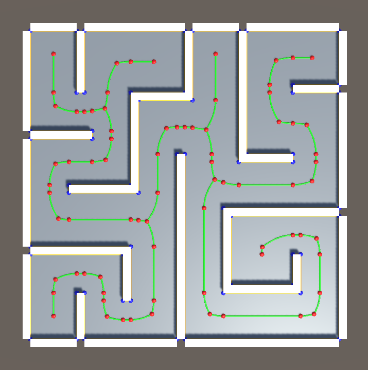
Polygonal Skeleton
We then apply a dilation of the skeleton to achieve two advantages, from [1]:
“First, the sharp angles between segments of the diagram are
smoothed, which improves the continuity of the generated trajectories and
frees them from sharp angles. Second, the Voronoi Diagram is thickened in
order to eliminate excessive narrowing, and thereby to allow a better propagation of the wave front when applying the Fast Marching Method.”
This skeleton represents the safest path through the maze, and for each pixel in our grid, set a viscosity as either a low or high value depending on the distance to this skeleton. Thus, assign a viscosity to each pixel according to:
(2) 
The particular viscosity values and the distance cutoff of 0.25 units were arbitrarily chosen, but seem to work well. This is visualized below:
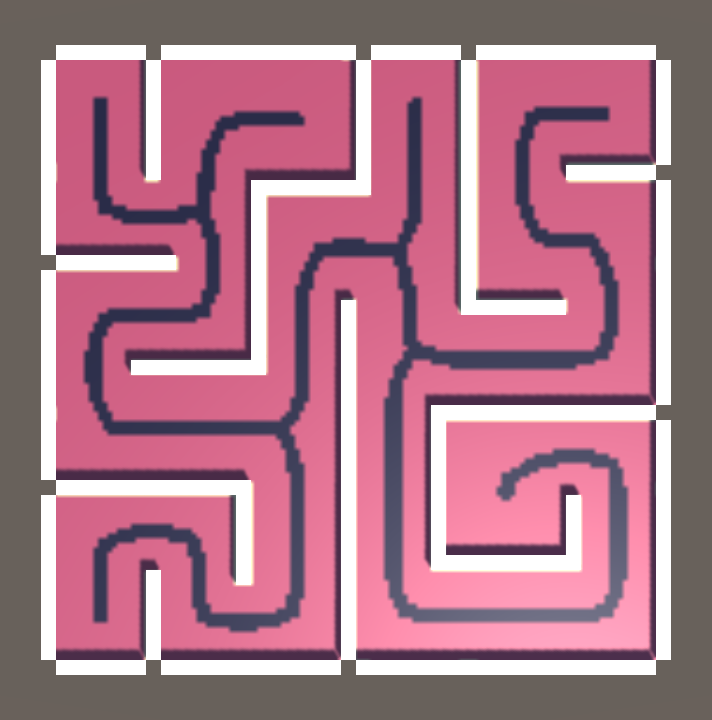
Viscosity Map
By setting the viscosity lower along the skeleton, the pseudo-wave will propagate until it reaches this path, and then race along it until it gets near to the robot’s location. Thus, the Fast Marching method will seek out the safe path along the skeleton.
Fast Marching Method
The Fast Marching method is a special case of more general level set methods, and is similar to Dijkstra’s algorithm in that it determines a path by projecting out from a front of accepted values. The method is as follows:
- Assign an arrival time of
 to every grid point and add them to a list of far points. Assign an arrival time of 0 to points on the boundary, and move them to a list of accepted points
 - For each of the four pixels adjacent to each accepted pixel, calculate a tentative arrival time via the Eikonal update, and move these pixels to a list of considered points
- Over all considered points, find the pixel with the minimum arrival time and move it to the accepted list
- For each of that minimum pixel’s neighbors that are not already accepted, use the Eikonal update to calculate an arrival time and move them to the considered list if necessary
- If the considered list is not empty, return to step 3
This method essentially advances a front of considered points, and then accepts them one pixel at a time. The Eikonal update is a first order scheme to approximate the partial derivative of u, with care taken to deal with missing neighbors or values of infinity for far points. From [3], for the grid point at  , let:
(3) 
(4) 
If  , then
(5) 
Solving for  :
:
(6) 
If  , then assuming one derivative is zero:
(7) 
The progression of the Fast Marching method is shown below. Earlier arrivals are darker and purple, later arrival times are brighter and yellow.
Fast Marching Method
Fastest Path
Once we have the arrival time for each point in the grid, we can determine the fastest path from the robot’s location to destination source. I originally tried implementing a 2D gradient for a steepest descent, but ran into issues with step size and toggling back and forth between pixels. Instead, I settled on a simpler approach that just moves to the pixel neighbor with the lowest arrival time. The path only moves from grid point to grid point and is thus not very smooth, but this method works well enough as a demonstration. An example path is shown below.
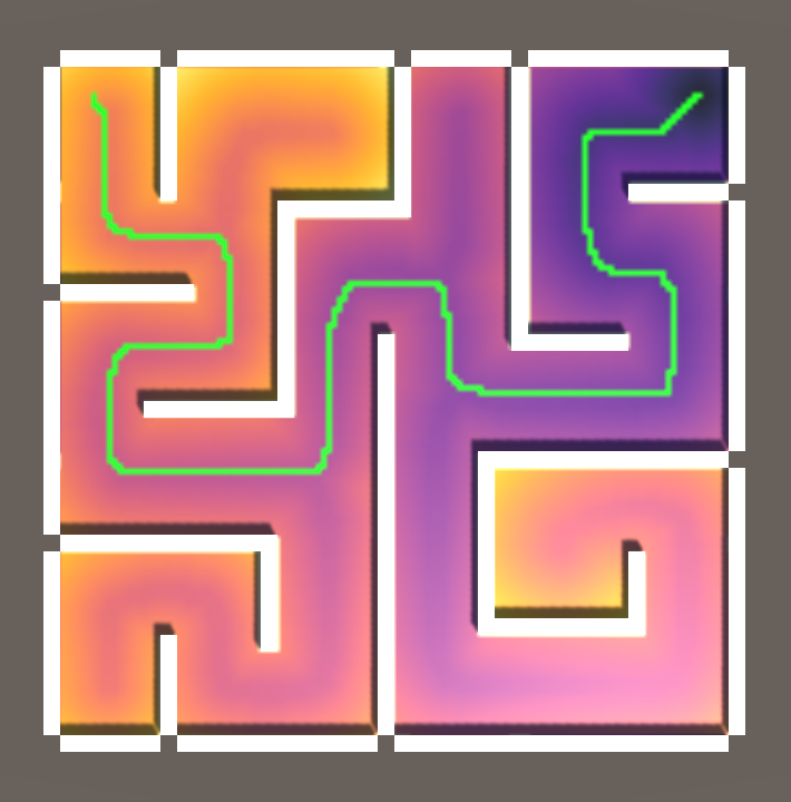
Example Path
References
- Garrido, Santiago & Moreno, Luis & Blanco, Dolores & Jurewicz, Piotr. (2011). Path Planning for Mobile Robot Navigation using Voronoi Diagram and Fast Marching. International Journal of Robotics and Automation. 2. 154-176.
- Sunday, D. Inclusion of A Point in a Polygon. http://geomalgorithms.com/a03-_inclusion.html
- Eikonal Equation. https://en.wikipedia.org/wiki/Eikonal_equation