A Weighty Matter

Removing Weights From a Barbell

One of the hobbies that I have taken up over the past few years has been lifting weights. I mostly follow powerlifting style routines, and those tend to involve relatively long rests between sets which leaves a lot of idle time. During one such break recently, I began to ponder the different orders one could remove the weights from a barbell.

One mistake people have to make at least once is to absentmindedly remove all of the weights from one side of the bar. This works up to a point, but if there is enough weight on the other side, the bar will dramatically tip over and the weights will come crashing down. As a practical matter, you can get away with a difference of two 45 lb plates between the sides, though a difference of three plates spells disaster. The general advice to avoid this is to simply remove the weights from alternating sides, keeping the center of gravity between the supports. To be impractical, given that you start with n plates on each side, how many ways can you remove them, both safely and unsafely?

Unconstrained Problem

Let’s tackle the simpler problem first, where we ignore physics and don’t restrict how unbalanced the bar can be. Given n weights on each side, let $U_n$ be the total number of ways to remove them. Label weights on each side $L_1, L_2, ... L_n$ , and $R_1, R_2, ... R_n$ , going from the outside in. Below is an example for $n = 3$ :

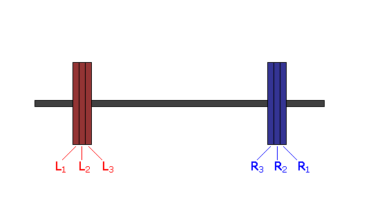
For this case, we can simply list all twenty possible removal orders by inspection:

L1, L2, L3, R1, R2, R3
L1, L2, R1, L3, R2, R3
L1, L2, R1, R2, L3, R3
L1, L2, R1, R2, R3, L3
L1, R1, L2, L3, R2, R3
L1, R1, L2, R2, L3, R3
L1, R1, L2, R2, R3, L3
L1, R1, R2, L2, L3, R3
L1, R1, R2, L2, R3, L3
L1, R1, R2, R3, L2, L3
R1, L1, L2, L3, R2, R3
R1, L1, L2, R2, L3, R3
R1, L1, L2, R2, R3, L3
R1, L1, R2, L2, L3, R3
R1, L1, R2, L2, R3, L3
R1, L1, R2, R3, L2, L3
R1, R2, L1, L2, L3, R3
R1, R2, L1, L2, R3, L3
R1, R2, L1, R3, L2, L3
R1, R2, R3, L1, L2, L3

If we were to list all the permutations of the six plates, there would be 6! = 720 possible combinations. But, notice that even though the left right order changes, we always take off the plates from the outside first, so L1 always precedes L2 which always precedes L3. For each of the listed orders, you could permute the three left plates in 3!=6 ways, and the three right plates in six ways. Thus, each of the listed orders corresponds to 36 of the 720 total combinations. Generalizing this observation, there are a total of

(1) $\begin{equation*} U_n = \frac{2n!}{n!n!} =\left(\begin{array}{c} 2n \\ n \end{array}\right)\end{equation*}$

possible unconstrained orders. Given 2n slots, we essentially choose where to place the n left (red) plates. That was easy!

Constrained Problem

Things get more complicated when we restrict how unbalanced the loading can be. At any point in time, define a signed delta loading by the number of plates still on the bar:

(2) $\begin{equation*}\Delta = n_L - n_R\end{equation*}$

We always start out with $\Delta=0$ , and we end up there as well. For a particular removal order, let $\Delta_{max}$ be the maximum value that $\lvert \Delta \rvert$ reaches at some point during the process, and let $C_n^m$ be the number of ways to remove n plates that have $\Delta_{max}$ exactly equal to m. It’s clear the minimum and maximum of $\Delta_{max}$ are 1 and n respectively, and these are the easiest cases to count directly.

If we limit $\Delta_{max}$ to 1 (the physically safe option, and what you should do in practice), we can think of each pair of plates as joined, and we simply choose one of two orders, LR or RL, for each independently. Thus, there are a total of $2^n$ removal orders with a $\Delta_{max} = 1$ :

(3) $\begin{equation*}C_n^1 = 2^n\end{equation*}$

The number of removal orders with $\Delta_{max} = n$ is even simpler. To reach that $\Delta$ , you have to remove all of the plates on one side before removing any from the other, so it’s literally just a choice between two orders: LL…LRR…R and RR…RLL…L

(4) $\begin{equation*}C_n^n = 2\end{equation*}$

For our example problem with three plates, that means $C_3^1=8$ and $C_3^3=2$ , from which we can deduce that $C_3^2=10$ . That works for this small case, but how can we calculate these medial values directly? To answer this, let’s introduce a way to visualize removal orders.

Removal Order Graph

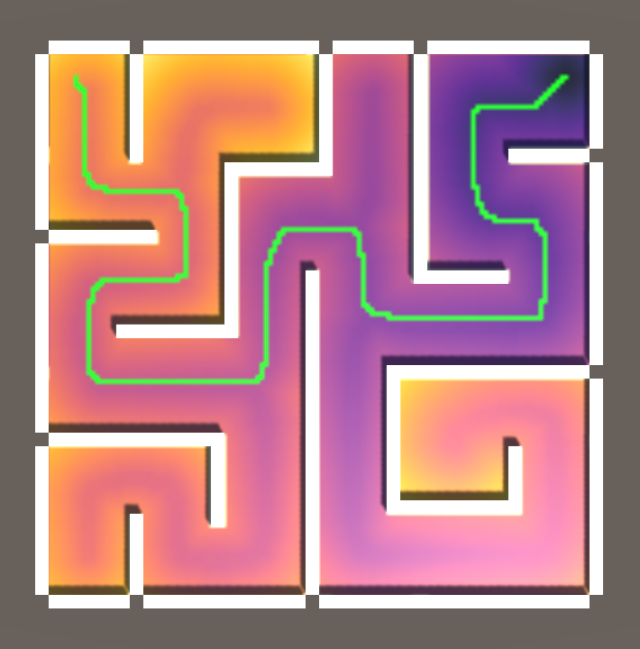
The graph below shows a potential order to remove weights with n=4. We start in the upper left corner with four weights on each side. If we remove a weight from the right side of the bar, we travel right on the graph, and if we remove a weight from the left side, we travel down. The path always starts on the upper left corner and always terminates at the lower right corner. Since we don’t add plates back to the bar, we can never travel left or up on the graph.

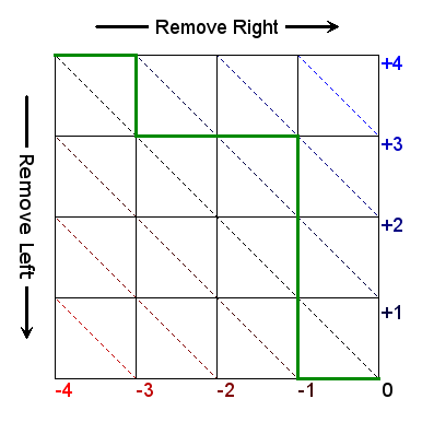
Particular values of $\Delta$ correspond to the labeled diagonals. For the case of the example path shown in green, $\Delta$ reaches a high of 2 before doing down to a low of -1, thus making $\Delta_{max} = 2$ for this path.

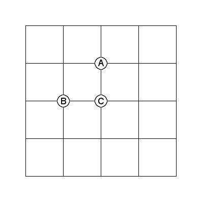
Since paths on this graph travel in only two directions, to arrive at node C, you would have to first path through either node A or node B. This means that if we know the number of paths that go through both nodes, $p_A$ and $p_B$ , then we can simply sum them to get the number of paths that go through node C:

(5) $\begin{equation*}p_C = p_A + p_B\end{equation*}$

We can easily do this for all the nodes in the graph, with the initial condition that there is one way to get to the starting node. For the unconstrained case we have:

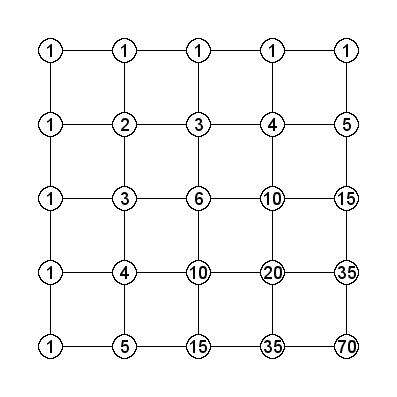
Since we can’t travel up, the nodes along the top of the graph inherit the number paths from the node to the left. This corresponds to just taking all the plates from the right side one by one. Similarly for the left side. So, by summing the nodes on the graph, we conclude there are 70 ways to remove four plates. This matches our earlier calculation from eq. 1. Observant readers will notice this is just a truncation of Pascal’s triangle. Individual nodes in the triangle can be calculated directly via binomial coefficients, due to the identity:

(6) $\begin{equation*}\left(\begin{array}{c} n \\ k \end{array}\right) = \left(\begin{array}{c} n-1 \\ k-1 \end{array}\right) + \left(\begin{array}{c} n-1 \\ k \end{array}\right) \end{equation*}$

Which can be seen as another way of arriving at eq. 1.

Instead of directly calculating $C_4^3$ , we can instead calculate all the paths with $\Delta_{max}$ less than or equal to three. Denote this by:

(7) $\begin{equation*}S_4^3 = C_4^1 + C_4^2 + C_4^3 =\sum_{i=1}^3 C_4^i\end{equation*}$

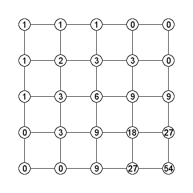
We can represent this on our graph by simply setting unreachable nodes to zero, i.e. setting the upper right and lower left nodes to zero:

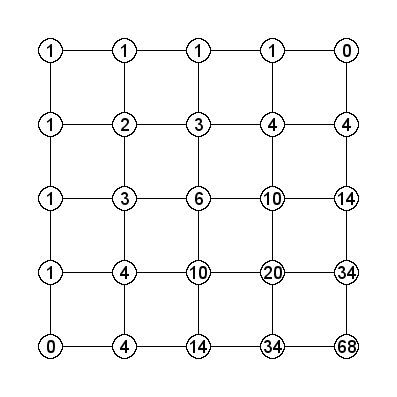
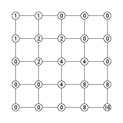
Which means there are a total of 68 ways to remove four plates without letting $\Delta_{max}$ exceed three. Similarly, limiting it to a two plate difference gives:

And hence, $S_4^2 = 54$ , and we can conclude that:

(8) $\begin{equation*}C_4^3 = S_4^3 + S_4^2 = 68 - 54 = 14\end{equation*}$

And finally, when we limit the differential to one plate:

Which validates the result from eq. 3.

Recursive Solution

The unconstrained problem had a compact answer in eq. 1, but I can’t see any concise way to describe the solution described above using binomial coefficients. However, we can describe the answer recursively. Label the nodes following the order of binomial coefficients in Pascal’s triangle:

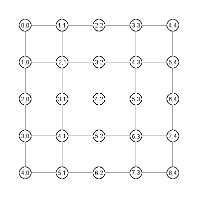
Let $S(n,k,m)$ be the value of node $(n,k)$ with the constraint that $\Delta_{max} <= m$ . We can calculate $\Delta$ directly for each node:

(9) $\begin{equation*}\Delta = 2k-n\end{equation*}$

And thus we can recursively calculate:

(10) $\begin{equation*}S(n,k,m) = \left\{\begin{array}{ll}0 & ,\left| \Delta \right| > m \\1 & ,k=0 \textrm{ or } n \\S(n-1, k, m) + S(n-1, k-1, m) & ,\textrm{otherwise}\end{array} \right.\end{equation*}$

And now we have a method to solve our very pressing problem!

Published by mikebrasher on October 26, 2019 | Permalink

Fast Marching Method

This is part 2, and you can read part 1 here. The source code for this project is on my github, and you can play around with the finished project here.

Eikonal Equation

With our Voronoi diagram in hand, we can now use it to help direct the Fast Marching method as in [1]. Conceptually, our destination is taken as a point source for sound or radio, which would of course propagate according to the wave equation. The front of these waves can be described by the Eikonal equation:

(1) $\begin{equation*} \begin{array}{@{} c r @{}} \lvert \nabla{u(x)} \rvert = 1 / f(x) & ,x \in \Omega \\ u(x) = 0 & ,x \in \partial \Omega \end{array} \end{equation*}$

To help make visualization easier, we discretize the maze into an evenly spaced 128×128 grid with spacing h, data over which can be stored as a texture in Unity. We then solve the Eikonal equation to determine how long it takes our pseudo-wave to reach each grid point, and then use that field to determine the quickest path from the robot’s current location to the destination. However, if we assume that the wave speed f is constant everywhere, this will lead a path that hugs the corners of the maze. This is where the Voronoi diagram comes in.

First take the full diagram and extract a skeleton of the input polygon. To do this, we define a signed distance function to the edge of polygon, with positive distances inside the polygon, and negative distances outside. This is done via the simplified winding algorithm using code adapted from [2]. This method basically just tracks upward and downward crossings of each edge of the polygon, and if they’re equal, the point is outside the polygon. Then we can remove any node from the diagram that has a signed distance function less than some small positive tolerance. This removes nodes outside the polygon and on its perimeter. The skeleton for our example maze is shown below.

Polygonal Skeleton

We then apply a dilation of the skeleton to achieve two advantages, from [1]:

“First, the sharp angles between segments of the diagram are
smoothed, which improves the continuity of the generated trajectories and
frees them from sharp angles. Second, the Voronoi Diagram is thickened in
order to eliminate excessive narrowing, and thereby to allow a better propagation of the wave front when applying the Fast Marching Method.”

This skeleton represents the safest path through the maze, and for each pixel in our grid, set a viscosity as either a low or high value depending on the distance to this skeleton. Thus, assign a viscosity to each pixel according to:

(2) $\begin{equation*} \nu = \left\lbrace \begin{array}{@{} l c @{}} 1 & ,d(p) < 0.25 \\ 10 & ,d(p) >= 0.25 \end{array} \right \end{equation*}$

The particular viscosity values and the distance cutoff of 0.25 units were arbitrarily chosen, but seem to work well. This is visualized below:

Viscosity Map

By setting the viscosity lower along the skeleton, the pseudo-wave will propagate until it reaches this path, and then race along it until it gets near to the robot’s location. Thus, the Fast Marching method will seek out the safe path along the skeleton.

Fast Marching Method

The Fast Marching method is a special case of more general level set methods, and is similar to Dijkstra’s algorithm in that it determines a path by projecting out from a front of accepted values. The method is as follows:

Assign an arrival time of $+\infty$ to every grid point and add them to a list of far points. Assign an arrival time of 0 to points on the boundary, and move them to a list of accepted points
For each of the four pixels adjacent to each accepted pixel, calculate a tentative arrival time via the Eikonal update, and move these pixels to a list of considered points
Over all considered points, find the pixel with the minimum arrival time and move it to the accepted list
For each of that minimum pixel’s neighbors that are not already accepted, use the Eikonal update to calculate an arrival time and move them to the considered list if necessary
If the considered list is not empty, return to step 3

This method essentially advances a front of considered points, and then accepts them one pixel at a time. The Eikonal update is a first order scheme to approximate the partial derivative of u, with care taken to deal with missing neighbors or values of infinity for far points. From [3], for the grid point at $x_{ij}$ , let:

(3) $\begin{equation*} U_H = \min \left( U_{i-1,j}, U_{i+1,j} \right) \end{equation*}$

(4) $\begin{equation*} U_V = \min \left( U_{i,j-1}, U_{i,j+1} \right) \end{equation*}$

If $\lvert U_H - U_V \rvert \leq h \nu_{ij}$ , then

(5) $\begin{equation*} \left( \frac{U_{ij} - U_H} { h } \right) ^2 +\left( \frac{U_{ij} - U_V} { h } \right) ^2 = \nu_{ij}^2 \end{equation*}$

Solving for $U_{ij}$ :

(6) $\begin{equation*} U_{ij} = \frac{U_H + U_V}{2} + \frac{1}{2} \sqrt{ \left( U_H + U_V \right)^2 -2 \left( U_H^2 + U_V^2 - h^2 \nu_{ij}^2 \right) } \end{equation*}$

If $\lvert U_H - U_V \rvert \geq h \nu_{ij}$ , then assuming one derivative is zero:

(7) $\begin{equation*} U_{ij} = \min \left( U_H, U_V \right) + h \nu_{ij} \end{equation*}$

The progression of the Fast Marching method is shown below. Earlier arrivals are darker and purple, later arrival times are brighter and yellow.

Fast Marching Method

Fastest Path

Once we have the arrival time for each point in the grid, we can determine the fastest path from the robot’s location to destination source. I originally tried implementing a 2D gradient for a steepest descent, but ran into issues with step size and toggling back and forth between pixels. Instead, I settled on a simpler approach that just moves to the pixel neighbor with the lowest arrival time. The path only moves from grid point to grid point and is thus not very smooth, but this method works well enough as a demonstration. An example path is shown below.

Example Path

References

Garrido, Santiago & Moreno, Luis & Blanco, Dolores & Jurewicz, Piotr. (2011). Path Planning for Mobile Robot Navigation using Voronoi Diagram and Fast Marching. International Journal of Robotics and Automation. 2. 154-176.
Sunday, D. Inclusion of A Point in a Polygon. http://geomalgorithms.com/a03-_inclusion.html
Eikonal Equation. https://en.wikipedia.org/wiki/Eikonal_equation

Published by mikebrasher on November 7, 2018 | Permalink

Voronoi Diagram

This is part 1 and you can read part 2 here. The source code for this project is on my github, and you can play around with the finished project here.

Overview

There are several algorithms that perform path planning given some sort of graph representation of the problem space, such as A*, Dijkstra, etc. However, when determining paths for robot navigation, this graph may not exist, so it is useful to begin by extracting a Voronoi Diagram to define the safest areas furthest away from obstacles, then obtain the actual path using the Fast Marching method, as noted in Garrido et. al. [1]:

“The method combines map-based and sensor-based planning operations to provide a reliable motion plan, while it operates at the sensor frequency. The main characteristics are speed and reliability, since the map dimensions are reduced to an almost unidimensional map and this map represents the safest areas in the environment for moving the robot.”

All code for this project can be found on my github page {x}.

Voronoi Diagram

The Voronoi diagram of a set of points in 2D defines planar regions that are closest to each point according to some distance metric, usually Euclidian distance. Several algorithms have been proposed to solve this problem; including Fortune’s advancing front algorithm, and generating the dual of a Delauney triangulation. Beyond Voronoi diagrams of points, generalized Voronoi diagrams define similar regions for line segments, arcs, and even three dimensions. This project generates 2D generalized Voronoi diagrams for sets of point and line segments following the method of HeHu09 [2].

In summary, staring from an initial diagram, each point site is added sequentially generating intermediate diagrams, then each line site is added sequentially. This method follows the incremental topology-oriented approach of Sugihara and Iri [3], which makes the algorithm reliable on floating point arithmetic, and the algorithm executes quickly in O(n log n) time.

The first step in this implementation is to extract a closed defining polygon from an input array of cube primitives which define the maze shown above. This is done in an ad-hoc way assuming the blocks are directly adjacent each other and do not overlap. This method which probably would not be robust in general, but works well for the given inputs. This simple closed polygon is then taken as the direct input to the Voronoi diagram.

Each vertex of the polygon shown below is taken as a point site, and each edge of the polygon is taken as a line site. Based on the bounding box of these, four dummy Voronoi noides are placed outside, along with one dummy site in the center.

Closed Defining Polygon

From [2]

“We require the Voronoi diagram under construction to fulfill the following topological conditions:

Every site has its own Voronoi cell
Every Voronoi cell is connected
The Voronoi cell of an open line segment [] is adjacent to the Voronoi cells of its endpoints”

Point Sites

At any point in time, the current Voronoi diagram will consist of Voronoi nodes which are equidistant to at least three sites, and Voronoi edges which are equidistant to exactly two sites and connect the nodes together. For any point, define a clearance disk as the closed disk centered at p whose radius is the smallest distance to any site. Each site, s, is then added incrementally via the following method:

Find the Voronoi seed node which whose clearance disk is most violated by s, i.e. maximize CD(seed) – dist(seed, s)
Recursively descend a depth-first tree to find other nodes whose clearance disks also cover s, and delete the edges connecting them
For each edge spanning the new Voronoi cell, calculate the intersection point between the edge and the bisectors of s and the edge’s sites, and make these intersection new nodes
Connect these hanging nodes with edges to define the new cell

When adding point sites, step 3 doesn’t require using both bisectors of the edge and the site, but it will be helpful when we get to adding line sites. In any case, each bisector should intersect the edge at the same point, but it is only added once. The bisector between any two point sites will just be the line going through the midpoint of the two sites, and the intersection of two lines is simple to calculate. An example of this step is shown below.

Three Point Sites

Starting with nodes s0 and s1, their bisector is shown as the dashed black line. An existing edge connects nodes n0 and n1 on this bisector. The clearance disk of n1 is show as the red circle, and the new point site to be inserted, s, lies within this clearance disk. The bisector of s and s0, and the bisector of s and s1 are both shown as the dashed blue lines. Each bisector intersects the previous edge at x. n1 is deleted from the node list, and a new node at x is added. The edge from n0 to n1 is deleted from the edge list, and a new edge from n0 to x is added.

Once all appropriate nodes have been deleted, and the remaining edges have been intersected with the new cell, all that remains is to connect these hanging nodes to form a topologically connect region. This happens as below, by matching the sites that define the edges together and calculating bisectors between these sites and s.

Connect A New Voronoi Cell

As each new node is created in the previous step, mark them as disconnected. As shown above, we are currently connecting node n3, which terminates edges e2 and e23. Edge e2 is defined by sites s and s2, edge e23 is defined by sites s2 and s3, and the node n3 is defined by all three sites. There is no edge currently in the edge list that is defined by sites s and s3, so we need to create it. We look through the disconnected node list to find node n4 which is also defined by s3, and generate an edge from n3 to n4 along the dashed blue bisector of s and s3. We then mark n3 as connected and continue with the next disconnected node, n4.

The algorithm is shown inserting all point sites for the example maze below. Point sites are shown as blue circles, Voronoi nodes as red circles, and Voronoi edges as green lines.

Inserting Point Sites

Line Sites

Inserting line sites proceeds following the same algorithm, just calculating the bisectors and intersections becomes a bit more involved. As noted before, the bisector of two point sites is a line. However, the bisector of a point site and a line site is a parabola, and it’s convenient to define this directly by its vertex an directrix, i.e. the point site and line site. Two line sites actually have a pair of bisectors, two lines that form an x. It’s simpler to intersect both bisectors with the current edge, and then throw out any intersections outside the line sites’ cones of influence. This zone is simply the set of points that lie within the line site when projected onto the underlying line.

The intersection of two lines is a single point, and unless they are parallel, will always exist. The intersection of a line and a parabola can be defined by a quadratic equation, and there can be 0, 1, or 2 solutions. As long as care is taken in the calculation, these can be taken directly from the exact solution. Generally two solutions will exist, but only one of these solution will be within the cone of influence of the line site.

The intersection of two parabolas is defined by a quartic equation, and even though analytic solutions exist, they are complicated and prone to numerical instability when calculating in floating point. One could implement a root finding algorithm such as Baristow’s method, but this appears to be unnecessary. In order to have two parabolic bisectors, we need to be currently looking at two line sites and one point site. However, we can just use the third bisector between the two line sites and calculate its intersection with either parabola. This is why earlier we considered both bisectors of the inserted site. Practically we implement the parabola-parabola intersection as an empty function that returns no intersection and rely on the other bisector to calculate it.

The algorithm is shown inserting all line sites for the example maze below. Additionally we split the parabolic edges at their apex to reduce cycles when descending the tree as in [2]

Inserting Line Sites

References

Garrido, Santiago & Moreno, Luis & Blanco, Dolores & Jurewicz, Piotr. (2011). Path Planning for Mobile Robot Navigation using Voronoi Diagram and Fast Marching. International Journal of Robotics and Automation. 2. 154-176.
Held M, Huber S. Topology-oriented incremental computation of Voronoi diagrams of circular arcs and straight-line segments. Computer Aided Design 2009; 41(5):327-38
Sugihara K, Iri M. Construction of the Voronoi diagram for ‘one million’
generators in single-precision arithmetic. Proc IEEE 1992;80(9):147184.

Published by mikebrasher on November 7, 2018 | Permalink